In this series we will use Vitis HLS to convert the linear values of our audio samples to the decibel scale used in digital audio processing, dBFS. In the first post we discuss how to convert our audio sample values from the linear scale to dBFS and take our first steps with Vitis HLS.
Linear Scale vs. dBFS
In a previous post we implemented an LED meter for visualizing the level of our audio signals with the LEDs on the ZedBoard. In that design we mapped eight ranges of the audio sample values to each of the LEDs using thermometer code. While that works fine, it has one potential for improvement: converting the sample values to dBFS (decibels Full Scale).
Decibels are used to represent ratios between two values. This is also the case in audio: If we say that the amplitude of a sine wave is 6 dB lower than the amplitude of another sine wave, it means that the amplitude of the first sine wave ist half that of the second sine wave. However, using dBFS we are also able to represent the absolute value of a digital audio signal. The conversion is done using the following formula:
sample_value_dbfs = 20*log10(abs(sample_value_linear)/max_value_linear)where:
- sample_value_dbfs is the value in dBFS for the corresponding audio sample in the linear scale
- sample_value_linear is the value of the sample in the linear scale
- max_value_linear is the (unsigned) maximum value that can be represented in the linear scale
For a 24-bit sample, max_value_linear is 8.388.608.
Using the formula above we find that the maximum amplitude in the linear scale is equivalent to 0 dBFS. Half the maximum amplitude in the linear scale (4.194.304) is equivalent to -6 dBFS, that is, halving any amplitud is equivalent to applying a -6 dB gain.
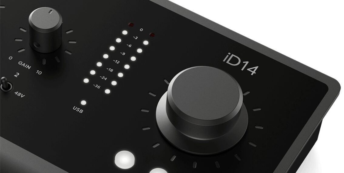
The figure below shows the LED peak meter on a desktop audio interface. The LEDs display levels between -36 and 0 dBFS, equivalent to 132950 and 8.388.608 in the linear scale.
Why Vitis HLS?
So how do we go about converting our audio sample values from the linear scale to dBFS? Our formula contains four operations: a multiplication, a log10, an absolute value and a division.
Three out of those four operations are easy to implement. We already learned how to extract an absolute value when we implemented the linear LED meter. The division is usually not a trivial operation for synthesis, but because we use a power of two as the divider, we can get away with a right shift. Because one of the operands in the multiplication is not a power of two, a shift cannot be used, but we can take advantage of the FPGA’s DSP blocks to directly perform the multiplication.
However, implementing a log10 operation on hardware is not trivial. One option is to design a custom digital circuit from scratch. Instead, we will use Vitis HLS.
The idea behind Vitis HLS (High-Level Synthesis) is that the designer provides a description of the functionality to be implemented on the FPGA fabric in a high(er)-level language like C or C++, and Vitis HLS will generate an RTL description that performs that function. The designer can also provide directives so that the tool optimizes for speed, latency, or resource utilization. Vitis HLS, much like C/C++ themselves, comes with a math library which includes – you guessed it – a log10 function.
Creating a Vitis HLS Project
Let’s set up our Vitis HLS project and load our design sources. We will need at least three files for a Vitis HLS project, namely:
- A header file that contains the declaration of our dBFS Converter function
- A source file that contains the definition of our dBFS Converter function
- A testbench file that contains the C/C++ Main function that will be used to test our dBFS Converter function
We will look at each of those files in detail in the next part of this series, for now we’ll focus on getting our project set up.
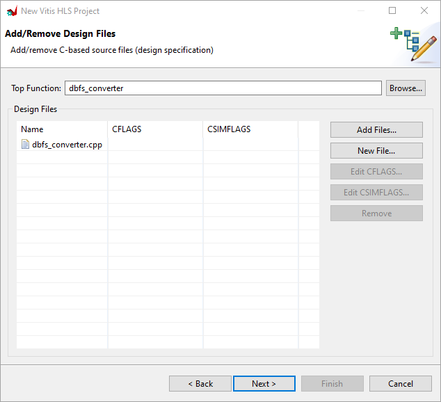
After starting Vitis HLS we are presented with the welcome screen, in which we select ‘New Project‘. In the following dialog we enter the project name and location. After that we add our source files and select the top-level function that we want to synthesize. This is shown in the figure below.
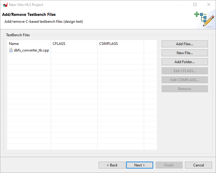
In the next window we add our testbench file, as shown in the figure below.
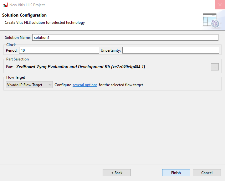
In the following window we set the solution configuration for our design as follows:
- Solution name: solution1. A solution is the result of the C/C++ synthesis performed by Vitis HLS given our C/C++ source files and a set of directives. A Vitis HLS project may contain several solutions for a single C/C++ description.
- Period: 10. This is the period, in nanoseconds, of the clock that drives our audio-processing logic.
- Uncertainty: This is a safety margin left by Vitis HLS so that it can be used by the Vivado place and route tools. The target clock period for the C/C++ synthesis will be the clock period entered previously minus the uncertainty, which is also specified in nanoseconds. If left blank, which we will for our project, the uncertainty defaults to 27% of the clock period.
- Part Selection: Select the ZedBoard under the ‘Boards‘ tab. This will load the correct part for our project.
- Flow Target: Vivado IP Flow Target. This will allow us to export the output of our Vitis HLS project and use it as an IP in our Vivado project.
Our Solution Configuration is shown in the figure below.
Now we are done setting up our project and are greeted by the Vitis HLS workspace, as shown in the figure below.
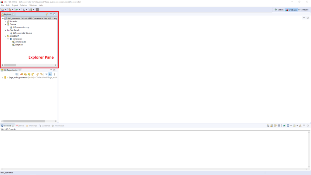
In the Explorer pane we see the files that we added when setting up the project. In addition to that, Vitis HLS has created two script files: script.tcl and directive.tcl. We will go over those files and the Vitis HLS simulation and synthesis workflow in the next post.
Vitis HLS Workflow
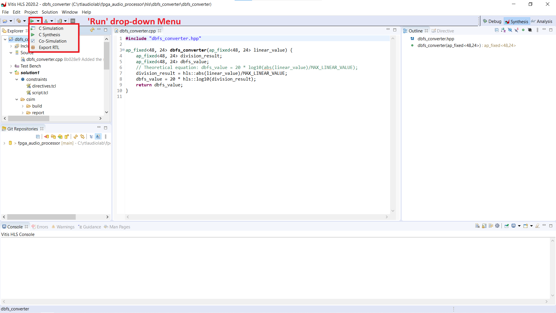
Now that our project is set up, we can start the Vitis HLS workflow to get to an RTL description. The Vitis HLS workflow has four steps, namely:
- C Simulation: In this step the correctness of the C/C++ description of our module is confirmed by running the testbench and checking the results. For small modules like the dBFS Converter this can be done by visually inspecting the module’s output, but it is a good idea to include automated checking in the testbench whenever possible.
- C Synthesis: In this step Vitis HLS generates the RTL representation of our C/C++ function. This is the core step in the high-level-synthesis process.
- Co-Simulation: In this step Vitis HLS runs the testbench from step 1, but instead of our C/C++ description, it uses the synthesized RTL to generate the output of the module. Here we can check that the RTL matches the C/C++ description.
- Export RTL: Once we have validated the RTL implementation, we need to export it so it can be instantiated as an IP in a Vivado project.
Each of these steps can be started from the ‘Run‘ drop-down menu in the Vitis HLS Workspace, as shown in Figure 6.
We will start with the C Simulation in the next post.
Cheers,
Isaac