035 – FPGA Floating-Point FIR Filter (2)

In this post, the second of a two-part series on the FPGA implementation of a floating-point FIR filter, we add support for stereo processing to our filter and listen to a processed audio sample.

In the first part of this series, we discussed and implemented the basic architecture of a floating-point FIR filter. You can read more about the use of floating-point processing in this project here.

Stereo Support

In the first installment of this series, we ended up with a working FIR filter engine, but to make it fully functional in our audio processor we needed to add stereo support. That’s what we are doing this time around, with a similar architecture as the one we used for the Limiter. Thus, the previous FIR Filter module, which can process a single audio channel, becomes the FIR Filter FSM module, two of which are instantiated in the new FIR Filter module. Compared to adding logic for reusing a single FIR Filter FSM module, this architecture is simpler and doubles the throughput of our FIR Filter, albeit at the expense of doubling the resource utilized.

The new description of the FIR Filter module is shown below.

module fir_filter # (
    parameter integer SP_FLOATING_POINT_BIT_WIDTH = 32
    ) (
    input   logic                                       i_clock,
    // Audio Input
    input   logic                                       i_data_valid,
    input   logic   [SP_FLOATING_POINT_BIT_WIDTH-1 : 0] i_data_left,
    input   logic   [SP_FLOATING_POINT_BIT_WIDTH-1 : 0] i_data_right,
    // Audio Output
    output  logic                                       o_data_valid,
    output  logic   [SP_FLOATING_POINT_BIT_WIDTH-1 : 0] o_data_left,
    output  logic   [SP_FLOATING_POINT_BIT_WIDTH-1 : 0] o_data_right
);

    timeunit 1ns;
    timeprecision 1ps;

    fir_filter_fsm  #(
        .SP_FLOATING_POINT_BIT_WIDTH    (SP_FLOATING_POINT_BIT_WIDTH )
    ) fir_filter_fsm_left_inst (
        .i_clock        (i_clock),
        .i_data_valid   (i_data_valid),
        .i_data         (i_data_left),
        .o_data_valid   (o_data_valid),
        .o_data         (o_data_left)
    );

    fir_filter_fsm  #(
        .SP_FLOATING_POINT_BIT_WIDTH    (SP_FLOATING_POINT_BIT_WIDTH )
    ) fir_filter_fsm_right_inst (
        .i_clock        (i_clock),
        .i_data_valid   (i_data_valid),
        .i_data         (i_data_right),
        .o_data         (o_data_right)
    );

endmodule

The FIR Filter FSM has the same logic as the old FIR Filter module from the first part of this series, but its IO signals have been updated to support a single channel.

Resource Utilization

The figure below shows the resource utilization of the floating-point FIR and IIR filters.

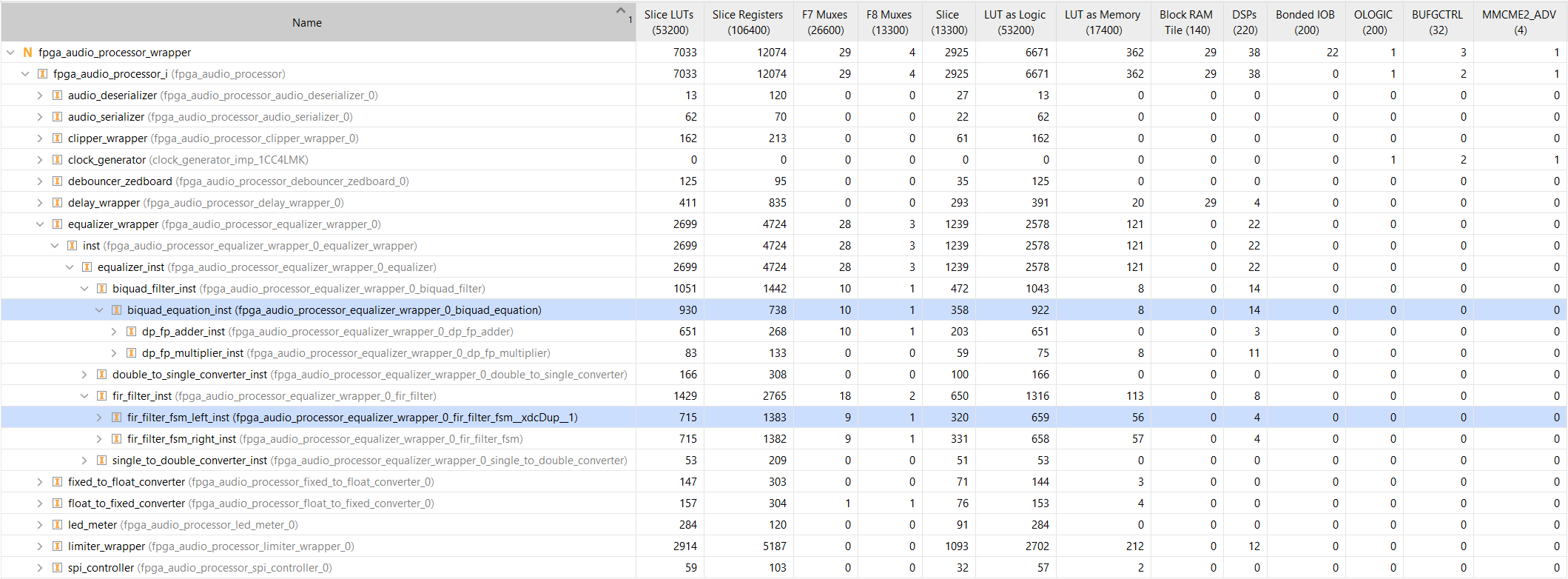
I’ve included the resource utilization numbers for the sake of completeness, but a direct comparison between the filters won’t be very meaningful. This is because the IIR filter uses double-precision floating-point processing, as opposed to the single-precision version of the FIR filter. Still, it may be useful to keep developing an intuition for the cost of these modules in terms of resources, especially when using floating-point processing.

Performance Analysis and Audio Samples

Now we get to the fun part. First, let’s check out the simulation of the IIR and FIR filters, to see how the output signal looks. Remember, we chose the coefficients so that they both implement a low-pass filter at about 500 Hz. The output of both filters is shown in the figure below.

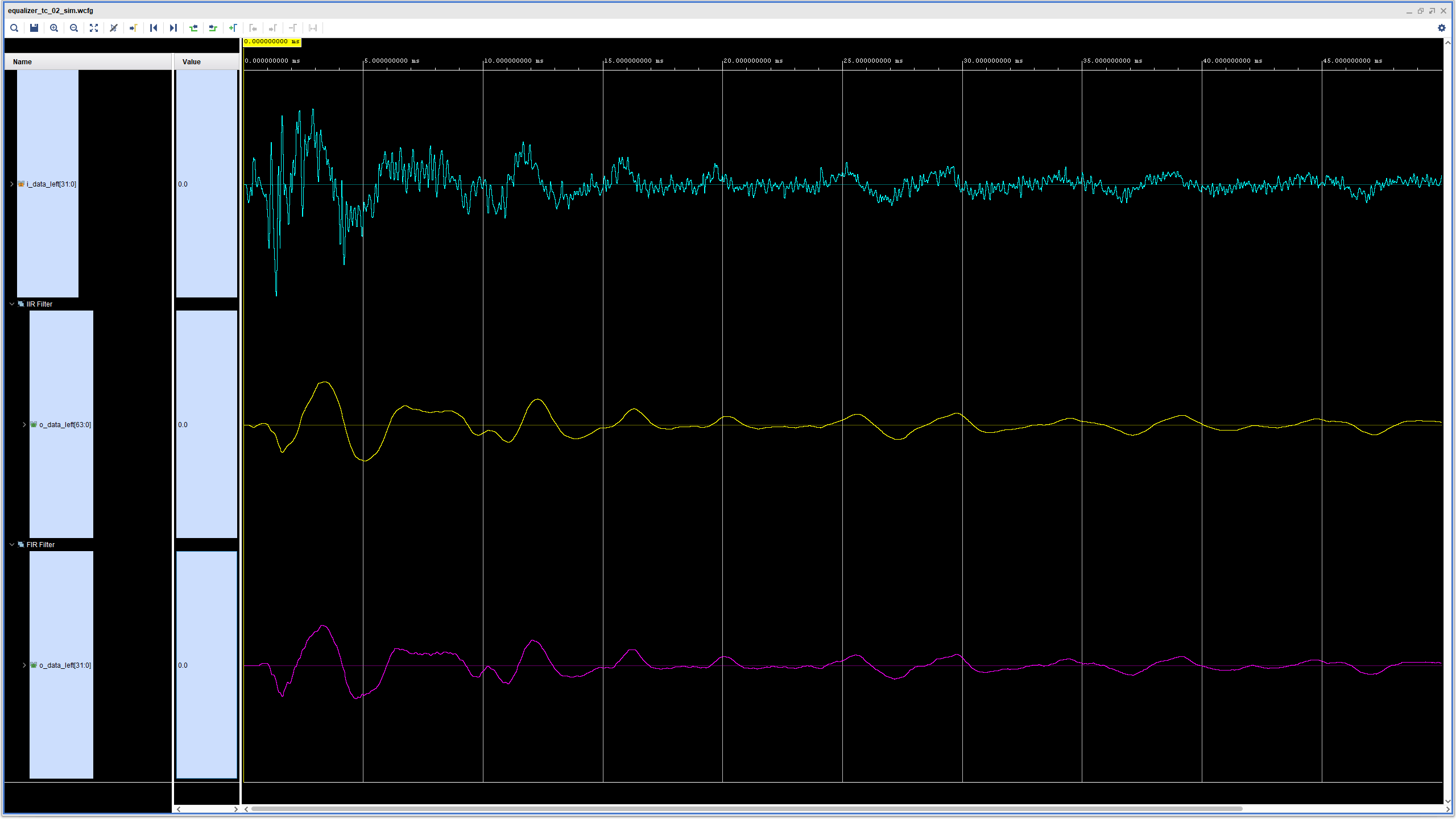
Now, the goal here is not to do a thorough analysis of the performance of each filter, but the waveforms do reveal that, as far as our goal of having one IIR filter and one IIR filter doing roughly the same processing goes, we seem to be in good shape.

A better way to evaluate the filter performance is to listen to it in action. The clip below plays four bars of unprocessed audio, followed by the same four bars processed by the IIR filter, and finally the same four bars processed by the FIR filter.

Finally, we want to be aware of the latency of our FIR filter implementation. The figure below shows the time elapsed between the arrival of an input sample and the generation of the corresponding output sample.

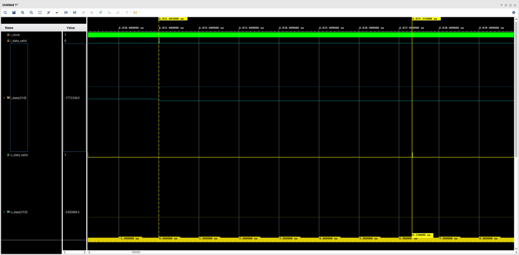
As we can see, it takes our implementation over 6 microseconds to generate the filtered output. This is enough for processing audio at 44.1, 48 and 88.2 kHz, but would exceed the time budget of a 192 kHz sampling rate by more than a microsecond. Moreover, this is a very naive implementation (even for floating-point standards!) that can be optimized.

One way to improve the performance of the filter would be to feed the data to the multiply-accumulate core as an AXI4-Stream. Triggering one operation and waiting for its output made sense (and was the only viable option) when implementing the IIR filter or the Limiter, because most operations depended on the value of the previous one. For the FIR filter, because the multiply-accumulate operation takes place within a single core, we could
have a continuous stream of data coming in, so that the core latency is only observed for the first sample, and we can get one output per clock cycle after that. This solution requires more logic to ensure compliance with the AXI4-Stream protocol at the input of the multiply-accumulate core, but the performance gains would make the effort well worth it.

That’s it for our exploration of floating-point FIR filters. In the next post we will do some cleanup and will introduce a non-project, script-based workflow for building our design.

Cheers,

Isaac

All files for this post are available in the FPGA Audio Processor repository under this tag. If you would like to support RTL Audio Lab, you can make a one-time donation here.